During my undergraduate course, I had the opportunity to do a presentation on the concept of FFT (Fast Fourier Transform), along with having to work with a DFT (Discrete Fourier Transform) price prediction algorithm during my internship experience. So today I’ll be covering what the FFT is, how it works, and why FFT is a DAC (Divide-and-Conquer) algorithm.

What and why FFT?

First I’ll explain FFT in terms of what you learn in Physics, as I believe this helps in understanding the individual steps and why those steps are necessary. I’ll cover the mathematical and algorithmic stuff later on.

FFT is a highly efficient algorithm that converts a signal from the time domain to the frequency domain. Okay…what? What does that even mean? To understand that, let’s first look at what signals are.

Understanding Signals

A signal describes how some physical quantity varies over time and/or space. Mathematically, it’s a function of one or more independent variables. A common example of a signal are sound waves, notably sine and cosine waves like below:

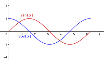
With the equations of sine and cosine waves being:

$$\begin{align} y(t) = A\ sin(\omega t + \phi)) + D \\ y(t) = A\ cos(\omega t + \phi)) + D \end{align}$$

where $A$ is the amplitude, $\omega$ represents angular frequency, $\phi$ is the phase shift, and $D$ is the vertical shift.

Here, the x-axis is commonly $t$ (referring to time) while the y-axis is the amplitude (the signal value at a given time $t$). Notice how the graph of sine and cosine are continuous values, meaning that they can take $t$ at any value. On the otherhand if they are discrete values where they can only take $n$ limited set of values, they would look like this:

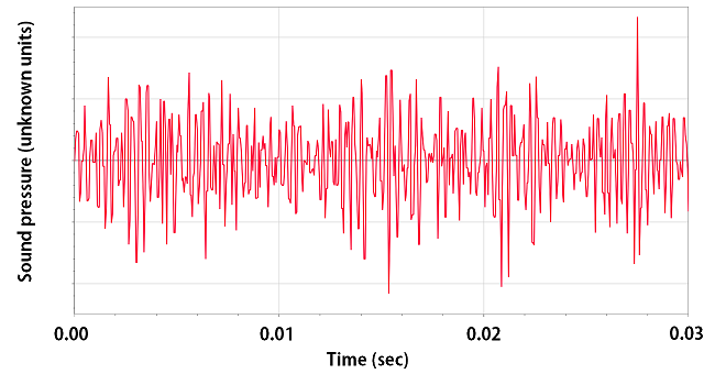
However the sine/cosine graphs would represent a extremely simple signal. In reality, different kind of signals are combined and mixed together as one input and would look much more chaotic like this:

Time and Frequency domains

We now have a basic understanding of what a signal is. Then what are time domain and frequency domain?

In math, a domain is the set of all possible input values you can put into a function (usually the represented as the x-axis of a graph) where the function $y = f(x)$ still produces a valid output. Thus a time domain, simply put, is just the domain of a function where it only takes time as the input of the function. All the graphs we have seen till now hence are graphs shown in the time domain. The time domain tells you the overall amplitude (the y value) over time.

The frequency domain, equivalently, takes frequency of the waves as its input values (x-axis) and has amplitude (the magnitude of the wave) as it’s y-axis (the output of the function). A signal drawn in the frequency domain would look something like this:

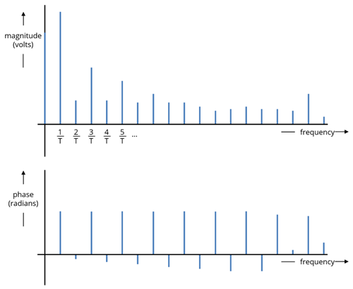
Notice how the frequency domain graph takes in discrete values.

The Fast Fourier Transform

Now we have all the building blocks to understand what the FFT does. Let’s go back to the definition of what an FFT is:

FFT is a highly efficient algorithm that converts a signal from the time domain to the frequency domain.

As mentioned earlier, an example of a signal is sound waves. Let’s say that you want to record yourself singing outside at a park on a beautiful warm summer day. Whatever mic you are using to record, the mic would not only pick up your voice, but also pick up every other sounds happening around you like birds chirping or the sound of cicadas, the sounds of other people talking, or sounds of water streams splashing and sloshing. All those sounds would be jumbled up into one chaotic signal (like shown earlier) fed into the mic. Since we want to only record your beautiful singing voice, we would want to be able to revert those combined sounds back into distinct individual signals; that’s exactly what the FFT does. FFT allows us to transition a signal from the jumbled up chaotic signal in the time domain where we can’t tell the different signals apart, into the frequency domain where we can distinguish those individual signals.

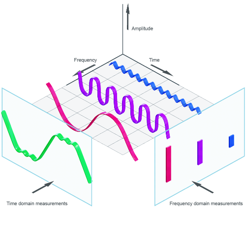
Perhaps its easier to understand visually. The graph below shows three different signals (blue, purple, and violet waves). From the perspective of time domain, the three signals are convoluted together into one signal (green wave), and we cannot tell apart the different signals hidden inside. But through FFT, we can transition our perspective to the frequency domain and distinguish the different waves.

Pretty cool huh? With this understanding, let’s look more deeply into the FFT as an algorithm and see how it does the magic. I’ll try to approach this in a top-down manner.

A deeper dive into the algorithm

Signals and waves can be represented as $d$-degree polynomials. The convolution of two waves can be represented as a product of two $d$-degree polynomials, resulting in a polynomial of degree $2d$.

Mathematically, if polynomials $A$ and $B$ are defined as $A(x) = a_0 + a_1 x + ... + a_d x^d$ and $B(x) = b_0 + b_1 x + ... + b_d x^d$, their product polynomial $C(x) = A(x) * B(x) = c_0 + c_1 x + ... + c_d x^d$ has coefficients

$$\begin{align} c_k = a_0 b_k + a_1 b_{k-1} + ... + a_k b_0 &\\ = \sum_{i=0}^k a_i * b_{k-i} &\\ (\text{for i > d, take } a_i\ \&\ b_i \text{ to be } 0) \end{align}$$

Computing this formula would take $O(k)$ steps, and finding all $2d + 1$ coefficients would require $\Theta(d^2)$ time.

FFT goes through the steps below and multiply polynomials in $O(n\ log\ n)$ time:

1. Input initialization: Start by taking $n$-points of the polynomial (the coefficients), where $n$ is a power of 2 (add padding if necessary). This is called the coefficient vector.
2. Decomposition: Split the coefficients into two $n/2$-points; one with all even-indexed samples and one with all the odd-indexed samples. This is applied recursively until you have $n$ single-point coefficients, which are their own FFTs (the base case).
3. Combining the coefficients: As the recursion unwinds, combine the results from the smaller FFTs. This combination is called the butterfly operation:
   • At each level, multiply the odd-indexed results by the twiddle factor (a complex number $W_N^k = e^{2\pi i k / N}$).
   • For the first half of the output, add these weighted odd-indexed results. For the second half of the output, subtract them (leverage symmetry to halve the work).
4. Final output: After combining at all stages, the resulting output is the polynomial evaluated at $n$ specific points (the roots of unity). We go through the inverse FFT (conjugate twiddles, divide by $n$) to get back the product polynomial’s coefficient.

Lets dissect the above step-by-step.

Step 1) Taking the signal as an input

Given a signal (a polynomial $P(x) = a_0 + a_1 x + a_2 x^2 + ... + a_{n-1} x^{n-1}$), the input is the coefficient vector $[a_0, a_1, ..., a_{n-1}]$, where $n$ is a power of 2.

Step 2) Decomposing the polynomial (and the magic of Roots of Unity)

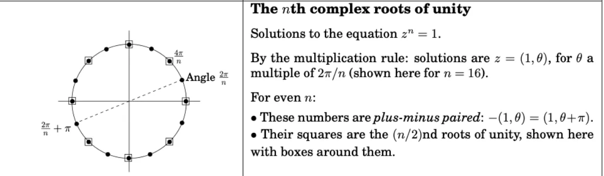
To evaluate the polynomial $P$ at $n$-th roots of unity, we need to recursively split and evaluate $P_{even}$ and $P_{odd}$ at the square of each roots. This is equivalent as evaluating the $n/2$-th roots of unity at two polynomials of degree $n/2 - 1$.

Below is a visual explanation of how roots of unity work.

Step 3) Combining the result

Once we reach the base case (if $n = 1$, return $a_0$), we start combining the results using the identity $P(x) = P_{even}(x^2) + x \cdot P_{odd}(x^2)$.

Set $w = e^{2 \pi i / n}$ (roots of unity $z^n = 1$). Then we evaluate $P(x)$ at $[w^0 = 1, w^1 = e^{2 \pi i /n}, w^2 = e^{2 \cdot 2\pi i /n}, ..., w^{n-1} = e^{(n-1) 2 \pi i /n}]$. I.e., for $k = 0,1,..., \frac{n}{2} - 1$,

$$\begin{align} y_k = P_{even} (w^{2k}) + w^k \cdot P_{odd}(w^{2k}) \\ y_{k + n/2} = P_{even} (w^{2k}) - w^k \cdot P_{odd}(w^{2k}) \\ \end{align}$$

The above subtraction works, and is one of the reasons that make FFT so efficient, through symmetry since $w^{k + n/2} = - w^k$ (representing halfway around the unit circle).

Step 4) Interpolation

After the forward FFT, we have the polynomial evaluated at the roots of unity—this is the point-value representation. To multiply two polynomials:

1. Compute FFT of both coefficient vectors
2. Multiply the results pointwise (element by element)
3. Apply the inverse FFT to recover the product’s coefficients

The inverse FFT is nearly identical to the forward FFT, with two modifications:

• Replace $w = e^{2 \pi i /n}$ with $w^{-1} = e^{- 2 \pi i /n}$.
• Divide the final result by $n$.

Mathematically, if the forward FFT computes $y_k = \sum_{j = 0}^{n-1} a_j w^{jk}$, then the inverse computes

$$a_j = \frac{1}{n} \sum_{k = 0}^{n-1} y_k w^{-jk}$$

This works because the roots of unity matrix is unitary (up to scaling), so its inverse is its conjugate transpose divided by $n$.

Divide-and-Conquer algorithm

Congratulations making it this far! If you have followed up till now, it should be fairly prominent how the FFT uses the Divide-and-Conquer strategy during its computation, which is also why the FFT algorithm is so efficient. As you guessed, step 2 of the algorithm divides the polynomials, and step 3 conquers by combining the polynomials back into one output. It’s as simple as that.

Below is the pseudocode of the algorithm as DAC:

PROCEDURE FFT(a, w):
	if w = 1: 
		return a
	(s_0, ..., s_{n/2 - 1}) = FFT((a_0, a_2, ..., a_{n-2}), w^2)
	(s'_0, ..., s'_{n/2 - 1}) = FFT((a_1, a_3, ..., a_{n-1}), w^2)
	for j = 0 ~ (n/2 - 1):
		r_j = s_j + w^j * s'_j
		r_{j + n/2} = s_j - w^j * s'_j
	return (r_0, ..., r_{n-1})

Final notes

FFT is one of the most important algorithms in modern technology and is widely used in different applications. Some common applications are in audio processing like equalization, noise cancellation, and MP3 compression, in image processing such as filtering, sharpening, and image compression, and in telecommunications like modulating/demodulating signals or identifying resonance frequencies in machineries.

As important as the FFT algorithm is, I remember I had an extremely hard time when I was learning about FFTs the first time. Even now I don’t think I can code the algorithm from scratch without referencing back to the notes I took in the past and without the help of internet. That being said, once you have truly understood a concept, even if you forget it it should be fairly easy to pick it back up later in the future. I hope this post helped you gain a deep intuitive understanding of how the FFT works and why it works, and can be used as a reference source for you to come back and review it whenever needed.

Lastly, below are couple of videos I’ve watched that helped me understand FFT when I was learning it myself. If you’re interested go take a look.

• (3Blue1Brown) But what is the Fourier Transform? A visual introduction (great visuals on how FFT works; highly recommended)
• (Reducible) The Fast Fourier Transform (FFT): Most Ingenious Algorithm Ever?
• (Veritasium) The Most Important Algorithm Of All Time