Introduction

Recently I finished reading Fundamentals of Data Engineering: Plan and Build Robust Data Systems by Joe Reis and Matt Housley, and went upon an important topic; the history of how data engineering evolved. The more I learn in technical topics like Computer Science, Software Engineering, and Data Engineering, I get the inclination that learning the history of how/why the common pattern of problems in that field emerge, and the evolution of different approaches in solving those problems, are critical. The problem patterns don’t change much despite how the field is always “rapidly changing”; it’s rather the solutions that change rapidly. So today I want to share the things I’ve learnt from that book.

Understanding this history helps explain why modern data stacks look the way they do, and why many “new” ideas are really just old ideas resurfacing at a different abstraction layer. Through this writing I hope readers can gain such understanding and apply this viewpoint not just in learning data engineering, but also in learning other technical fields as well.

The Evolution Timeline

1980s ~ 2000s: the Data Warehousing Era

As with most things in history, Data Engineering wasn’t really a thing back in the days. Bill Inmon, recognized by many as the “Father of Data Warehouse” first coined the term Data Warehouse (DW). In 1989, Bill defined Data Warehouse as

A subject-oriented, integrated, time-variant, and non-volatile collection of data in support of maangement’s decision making process.

It helps understand the technological and business environment at that time to understand why Bill defined DW as such. In 1970s, Edgar F. Codd published his paper A Relational Model of Data for Large Data Banks, introducing a new way to structure data in tables (or relations) using set theory and relational algebra. This led to the development of SQL (Structured Query Language) by IBM, and the further development of the first commercial RDBMS (relational database management system) by Oracle in 1979.

Soon after, RDBMS blew up; more and more companies were adopting those systems to collect, organize, and analyze company related data. There are several factors that made RDBMS and SQL such a hit at that time.

The Standard of SQL

The adoption of SQL as an ANSI standard (1986) and ISO standard (1987) created a universal language for anyone, albeit with some minor differences in detail between different vendors, interacting with the company’s data.

Data Integrity

RDBMS offered a strict guarantee of consistent clean data, preventing data corruption through ACID properties:

• Atomicty: A transaction is a all-or-nothing operation. Either all of its sub-routines occur successfully, or none do, preventing partial updates.
• Consistency: Ensures a transaction / operation to the data is always valid: upholding all rules, constraints, and triggers. This was important in preventing data to become corrupt or illogical.
• Isolation: Concurrent transactions didn’t interfere with each other, preventing issues like dirty reads or lost updates
• Durability: Once a transaction is committed (ran successfully), its changes are permanent and survives system failures like power outages and crashes. This was often done using transaction logs for recovery.

Hardware Advancements

The first major boom for commercial computers happend in 1980s, especially in the offices. Before that most things, including operations on business-critical data management, were done by hand manually and thus being more error-prone and slow in reporting and analysis. With the advancement of mainframes and computing hardware, corporations started leaning to incorporate on-premise servers in managing computations.

As companies started storing more and more data into relational databases, the volume of data started growing rapidly along with the emrgence of MPP (Massively Parallel Processing) databases. MPPs allowed companies to scale their analytical workloads. This established a core idea that still exists in Data Engineering today: separate operational systems from analytical systems, and design explicitly for analytics.

But a big limitation with these systems was that they were fundamentally centralized and monolithic. In other words, they scaled up vertically requiring more and more computational power.

Early 2000s: the Rise of Big Data

Another big reason that made companies move to RDBMS not mentioned above was the boom of internet in the late 1990s. However soon with the dot-com bubble burst happening in 2000, the surviving companies faced a new problem: traditional data warehouses were too expensive, too rigid, and too fragile for web-scale data. The requirement of web-scale data needing to be stored and analyzed started exploding uncontrollably, mainly along three dimensions: volume, velocity, and variety (this became the early definition of what defines “Big Data”).

Google’s response to this problem were a conceptual “big bang,” and it reshaped the industry for many years ahead. In 2003, Google released a paper on GFS (the Google File System) and soon after in 2004 published MapReduce: Simplified Data Processing on Large Clusters.

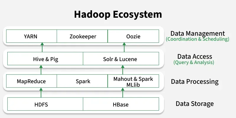
At the same time, significant technological advancements were made in computing hardware as well. Servers, RAM, and disks were starting to become more powerful and, most importantly, cheap and ubiquitous. This technological advancement in hardware allowed companies to easily build large clusters of computing nodes. Soon after in 2006, Hadoop made its first release to the open-source world, implementing the ideas residing in the papers Google has released, and allowing the problem of Big data to become engineerable.

I didn’t want this post to be technical, but the two concepts GFS and MapReduce are so pivotal in Data Engineering that they deserve some spot light. I’ll cover breifly on what they are and how they work; for those who aren’t really interested in the technical details, you can safely skip the rest of this section.

Intro to GFS

The GFS is a scalable, distributed file system designed to handle massive datasets on clusters of nodes, providing reliability and high aggregation performance. It primarily manages two types of data, the File metadata and File data. The GFS gains its efficient aggregation performance through the map-reduce method explained below. In the simple sense, it firsts distributes the data across nodes of machines, usually in the size of 64MB pieces. These chunks of data are split up and replicated across the network (by default replicates three copies).

The master node maintains a hierarchical directories across the cluster that keeps track of the metadata like namespace, access control, and the mapping of the data (paths of which the chunks of data reside).

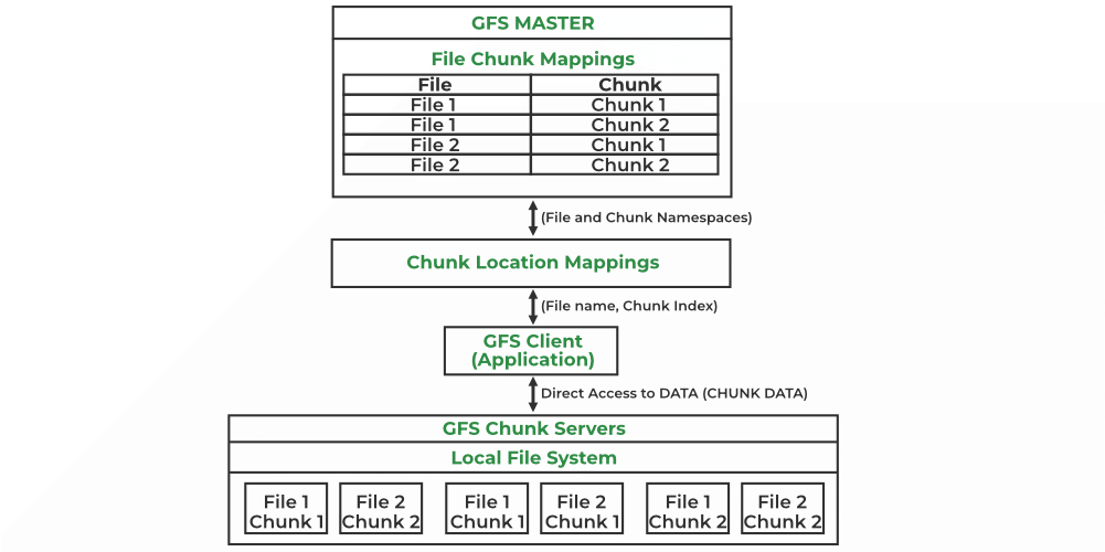
Above architecture enabled high availability and data recovery through replication, which is absolutely essential for the end-users. For example, let’s say a user is accessing a critical data that resides in multiple servers, but has no orchestrator like the GFS master node to point dynamically when needed. If the current server the user is requesting to goes down, then it required a manual intervention from the server side to point to the other server, which would inquire some latency to the end-user. However with the functionality of the master node, GFS can simply use the metadata to point to another redundant server immediately even if one server fails.

Intro to MapReduce

MapReduce nowadays is perhaps most commonly associated with the Hadoop framework to access the big data stored in Hadoop File System (HDFS). However in the pure sense, MapReduce is simply a programming model, or a pattern, of performing aggregated computation across a cluster of nodes. MapReduce first splits large amounts of data up to petabytes into smaller chunks. It then processes them parallely where the computation logic is executed on the server side where the data resides. Finally, it combines the results into one output to the user.

MapReduce, as the name suggests, has two main functions: Map and Reduce.

• During the Map phase it takes the initial data, dividing it into smaller chunks called “splits,” and assigns each split to a mapper as <key,value> pairs. This phase aims to filter, sort, and prepare the data for further computation, working in parallel for speed and scalability.
• During the Reduce phase is where the actual aggregation and summarization of data happens. It takes in the <key,value> pairs from earlier and “shuffle and sorts” them where pairs with the same keys are grouped together. Then it is sent to the reducer function, which receives a unique key and the list of values associated with it, and applies the user-defined computation logic (whether it be summing, averaging, filtering, etc.). The final output of all reducers are collected and written into a distributed storage system like GFS.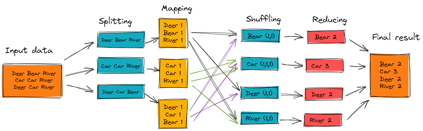

Late 2000s ~ 2010s: the fall of Big Data

With the release of Hadoop, the Hadoop ecosystem exploded as it offered a cost-effective, scalable, and open-source solution for storing and processing Big Data.

This era created the role of Big Data Engineer that requires a deep knowledge of distributed systems and comfortability with Hadoop cluster operations along with low-level tuning. They were responsible for keeping massive but fragile systems alive. But success came with a cost. As Big Data thrived, the Hadoop tooling sprawl increased complexity, and operating Hadoop clusters became a full-time job with costly operations on the business. With such caveats, the term “Big Data” itself became meaningless as people started realizing the size of data will just continue to grow and grow, and most importantly, at the end of the day it was just… data. Dan Ariely famously joked:

Big Data is like teenage sex: everyone talks about it, nobody really knows how to do it, everyone thinks everyone else is doing it, so everyone claims they are doing it.

At this point, the industry hit diminishing returns on complexity and investment on Big Data became obsolete.

2010s ~ Modern: Covering the Data Lifecycle

The modern data stack is a direct reaction to how much pain the Hadoop ecosystem caused.

From Monoliths to Modular Systems

Instead of one massive framework like the big complex Hadoop ecosystem, systems are now more decentralized, loosely coupled by default, and managed by the providing platforms (PaaS) like AWS (Amazon Web Services; AWS is IaaS, not PaaS). Some examples of these are cloud-native warehouses like Snowflake and BigQuery, along with managed streaming services like Kinesis, and specialized tools for ingestion, transformation, and orchestration like Airflow or Dagster.

From ETL → ELT pipelines

A central part of being a Data Engineer is building reliable data pipelines across different systems. Historically, the process of ETL data pipelines going through the stages of Extract → Transform → Load. This made sense because in the past warehouses were expensive, computing power was scarce, and thus transformations had to happen before loading. Cloud native data warehouses flipped those constraints as they became cheaper in storage, elastic in computing by separating storage layer and compute layer, leading to extremely fast SQL engines on massive datasets.

The change from centralized on-premise warehouses to decoupled cloud-native warehouses made the transition from ETL pipelines to ELT pipelines, going through the stages of Extract → Load → Transform (the Transform and Load stages are switched). We now load the raw data first from the cloud DW, transform the data within the same storage layer, the warehouse, and thus preserving a source-of-truth in the use of data for reuse and reprocessing. This wasn’t just a tooling change; it was an architectural decision.

Till now we have covered how the field of Data Engineering has evolved from the 1980s to modern era. As much as it’s important to know the history, I think it’s also as equivalently important as to keep an eye out on what’s coming ahead. What does the future of Data Engineering look like? Where are we heading towards now?

An Outlook to the Future

Some things are clear; data engineering and the data lifecycle isn’t going away anytime soon, perhaps forever as long as humanity thrives. The modern life is tightly intertwined with software and online interactions, and as time goes, more and more data will be stored and analyzed continuously. Abstraction of problems shifts responsibilities upward, it doesn’t remove them. Complexity is declining at the infrastructure level (as platform-managed services becoming more and more common), and increasing at the system design and governance level. Data Engineers are becoming increasingly aware of the importance of Data Governance: security, quality, and compliance must be designed from day one, and must maintain flexibility growing alongside the business itself.

Roles are also blurring: DE, SWE, ML, and analytics engineering are converging around operational ownership. A likely future role sits between ML engineering and data engineering, especially with the fast-growing AI and LLM workloads such as: monitoring pipelines and data quality, automating model training, and operationalizing end-to-end ML systems.

Data operations are becoming more cloud-native as well, with the rise of cloud data “operating system.” Data services are by default operating at cluster scale, and Warehouses, object storage, and streaming systems are starting to behave as a separate plug-and-play APIs like managed system calls of an operating system. With the need for higher-level orchestration, data APIs are becoming more standardized, file formats are becoming interooperable, Metadata catalogs are gaining popularity, and data-aware orchestrations from Airflow to Dagster are becoming the trend.

Another important trend is Real-Time Streaming. Batch processing is no longer the center of gravity as businesses require faster real-time insights. Just thinking about how social media platforms like Instagram, TikTok, and Youtube, require real-time algorithmic recommendations as the user quickly scrolls through video shorts. Historically, streaming was “hard mode.” But now that complexity is now moving down the stack with tools like Pulsar.

Final Thoughts

Every generation of data engineering tries to make the previous one obsolete. In reality, it just raises the abstraction level as the tools and constraints change throughout time. Through such changes, I always feel the need to go back to the start and focus on the fundamentals. At the end, data itself is not useful as-is; it only provides its use through some sort of action. We must go back and ask ourselves,

How do we reliably turn raw data into business value—at scale?

Thanks for reading my post.